1. Find and filter datasets

The catalog is a table with one row per dataset, and every search in the client is a filter on that table. The sections below show what the columns hold and how to select rows with exact facet values, numeric ranges, free text and genes. It also covers the mistakes that return the wrong datasets without an error, so that you can check a selection before you download anything.

You will learn how to:

• list the facets and their values, and count datasets per value

• combine facet filters and numeric ranges in query

• use search, and know when it returns more than query

• read the "did you mean" errors and use the aliases the client accepts

• select tissues and diseases, whose values are ontology terms

• find datasets that express a gene

• filter on quality and license

Nothing here downloads a dataset. Everything except the gene filter reads only the catalog file, which is about 7 MB.

import warnings

import matplotlib.pyplot as plt
import pandas as pd

import sddb

pd.set_option("display.max_colwidth", 60)

cat = sddb.Catalog(version="2026-10-28")
cat

<Catalog: 6087 datasets>

The catalog and its columns

Catalog(version="2026-10-28") reads the release of 28 October 2026, so the counts below stay the same when the catalog is updated. 0. Overview: from a query to a cited cohort explains why every tutorial pins the same release.

to_df() returns the whole table as a pandas DataFrame. The columns fall into a few groups, and the table below shows one example row for the columns you will use most.

df = cat.to_df()
print(df.shape)

groups = {
    "what was measured": ["organism", "tissue", "disease", "technology", "assay"],
    "how big it is": ["n_obs", "n_features", "size_bytes"],
    "where it comes from": ["study_id", "source", "collections", "doi"],
    "quality and terms": ["tier", "validation_status", "license"],
    "how to open it": ["uid", "slug", "zarr_url"],
}
example = df.loc[df["uid"] == "qEP9pd4LlyKeufe20000"].iloc[0]
pd.DataFrame(
    [(group, col, example[col]) for group, cols in groups.items() for col in cols],
    columns=["group", "column", "example value"],
)

(6087, 75)

	group	column	example value
0	what was measured	organism	human
1	what was measured	tissue	pancreas
2	what was measured	disease	pancreatic ductal adenocarcinoma
3	what was measured	technology	Visium
4	what was measured	assay	Visium Spatial Gene Expression
5	how big it is	n_obs	1142
6	how big it is	n_features	17943
7	how big it is	size_bytes	2577782
8	where it comes from	study_id	geo:GSM8915497
9	where it comes from	source	geo
10	where it comes from	collections	[geo-gse294669]
11	where it comes from	doi	10.1172/jci.insight.191595
12	quality and terms	tier	bronze
13	quality and terms	validation_status	pass
14	quality and terms	license	ncbi-geo-policy
15	how to open it	uid	qEP9pd4LlyKeufe20000
16	how to open it	slug	visium-spatial-gene-expression-pancreas-qep9pd4llykeufe2...
17	how to open it	zarr_url	s3://scverse-spatial-eu-central-1/.lamindb/qEP9pd4LlyKeu...

The example is a Visium section of a human pancreatic tumour from GEO. Its study_id is the GEO sample accession, and source is the prefix of study_id (geo), which the client derives when it loads the catalog. n_obs is the number of observations in the main table (spots here, cells for Xenium or MERSCOPE), and size_bytes is the size of the whole store, images included. Catalog columns describes every column.

Facets

A facet is a column you can filter on with an exact value. cat.facets() lists the facets, and with a column name it lists the distinct values of that column. From the shell, sddb-cli facets and sddb-cli facets technology print the same lists.

cat.facets()

['study_id',
 'doi',
 'organism',
 'tissue',
 'disease',
 'development_stage',
 'technology',
 'assay',
 'modalities',
 'tier',
 'validation_status',
 'license',
 'license_noncommercial',
 'hne_image',
 'if_image',
 'source',
 'preservation_method',
 'magnification',
 'collections']

cat.facets("technology")

['Atera',
 'CODEX',
 'CosMx',
 'MALDI-MSI',
 'MERFISH',
 'Merscope',
 'PhenoCyclerFusion1',
 'PhenoCyclerFusion2',
 'SpatialTranscriptomics',
 'Visium',
 'VisiumHD',
 'Xenium',
 'spatial-ATAC-seq',
 'spatial-CUT&Tag']

query() with no arguments returns every dataset as a cohort, and groupby counts the datasets per value of a column.

everything = cat.query()
print(everything)
everything.groupby("technology")

<SpatialDataCohort: 6087 datasets>

	technology	n
0	Visium	4022
1	Xenium	1234
2	SpatialTranscriptomics	552
3	VisiumHD	134
4	Merscope	115
5	MERFISH	10
6	spatial-CUT&Tag	4
7	MALDI-MSI	3
8	CosMx	3
9	Atera	2
10	PhenoCyclerFusion1	2
11	CODEX	2
12	PhenoCyclerFusion2	2
13	spatial-ATAC-seq	2

The left panel shows the same counts on a log scale, so that the technologies with two or three datasets stay visible next to Visium. The right panel shows the share of each curation tier per technology, which the section on quality explains.

tiers = pd.crosstab(df["technology"], df["tier"].astype("string").fillna("no tier"))
tiers = tiers.loc[tiers.sum(axis=1).sort_values().index, ["silver", "bronze", "no tier"]]
total = tiers.sum(axis=1)
share = tiers.div(total, axis=0)

fig, (left, right) = plt.subplots(1, 2, figsize=(10, 4.5), sharey=True)
left.bar_label(left.barh(total.index, total, log=True), fontsize=8, padding=2)
left.set_xlim(1, total.max() * 3)  # room for the labels
left.set_xlabel("datasets (log scale)")
start = 0
for tier, color in zip(share.columns, ["#8fa3b8", "#c08a52", "#cccccc"], strict=True):
    right.barh(share.index, share[tier], left=start, color=color, label=tier)
    start = start + share[tier]
right.set_xlabel("share of datasets")
right.legend(title="tier", frameon=False, ncol=3, loc="lower center", bbox_to_anchor=(0.5, 1.0))
fig.tight_layout()

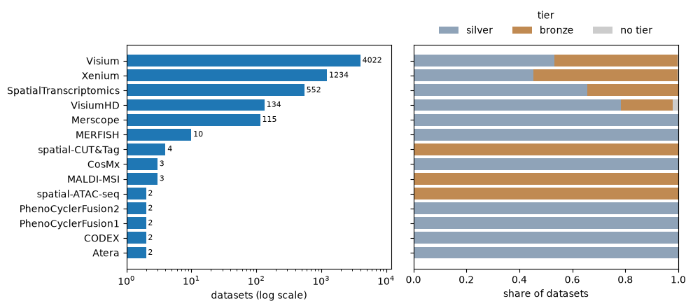
Visium and Xenium make up most of the catalog, and eight technologies have fewer than five datasets each.

Filter with query

query takes facet columns as keyword arguments. A single value keeps the rows equal to it, a list keeps the rows equal to any of its values, and several keywords must all hold.

lung = cat.query(organism="human", technology="Visium", tissue="lung")
lung

<SpatialDataCohort: 152 datasets>

lung_any_visium = cat.query(organism="human", technology=["Visium", "VisiumHD"], tissue="lung")
lung_any_visium.groupby("technology")

	technology	n
0	Visium	152
1	VisiumHD	6

The result is a SpatialDataCohort. It holds the matching catalog rows and nothing else, so building it takes no time and downloads no data. summary() gives the headline numbers, and to_df() returns the rows.

lung_any_visium.summary()

{'n_objects': 158,
 'n_studies': 157,
 'n_without_study_id': 0,
 'technologies': ['Visium', 'VisiumHD']}

n_studies counts distinct study_id values. For GEO data the study_id is the sample accession (GSM...), so a GEO series with ten samples counts as ten studies here. 3. Cohorts and manifests comes back to study ids when it groups datasets by study.

Numeric ranges

Append __gte, __gt, __lte or __lt to a numeric column to filter on a range. The numeric columns are listed in sddb._catalog_schema.RANGE_COLUMNS.

large = cat.query(organism="human", technology=["Visium", "VisiumHD"], n_obs__gte=50_000)
large.to_df()[["uid", "technology", "tissue", "n_obs"]].head()

	uid	technology	tissue	n_obs
0	haOzFbJ7Bc9x7NW60001	VisiumHD	ovary	475742
1	2TR7434o4LgFuwCi0000	VisiumHD	brain	521175
2	TfXXJl6p6e5ZtUxI0000	VisiumHD	tonsil	553820
3	wkdYCDgiAN7RJEZb0000	VisiumHD	lung	605471
4	k5Q3YIsLRHtzFqFR0000	VisiumHD	lung	448109

A row with a missing value never matches a range. n_features is missing for some datasets, so a range on it drops them even when you meant to keep every dataset:

print("rows without n_features:", int(df["n_features"].isna().sum()))
print("n_features >= 0:", len(cat.query(n_features__gte=0)), "of", len(cat))

rows without n_features: 663
n_features >= 0: 5424 of 6087

n_features__gte=0 looks like it keeps everything, but it returns 663 fewer rows than the catalog has. Check coverage() on a cohort, or isna() on the column, before you filter on a range.

Aliases and "did you mean" errors

Facet values are compared against the whole catalog before the filter runs. A value that is not in the catalog goes through a few aliases first. Case, spaces, hyphens and underscores are ignored, and technology also accepts the label in the assay column, which is what the website shows. The three calls below select the same datasets:

[len(cat.query(technology=value)) for value in ("Xenium", "xenium", "10x Xenium")]

[1234, 1234, 1234]

A value that still does not match raises a ValueError with the closest known value. The error is deliberate, because a typo used to return an empty result without any error.

for facet, value in [("technology", "Xenum"), ("tissue", "lungs"), ("organism", "Homo sapiens")]:
    try:
        cat.query(**{facet: value})
    except ValueError as err:
        print(err)

unknown technology value 'Xenum'; did you mean 'Xenium'?
unknown tissue value 'lungs'; did you mean 'lung'?
unknown organism value 'Homo sapiens'; list the values with facets('organism')

The last message has no close match, because organisms are stored by common name (human, mouse) and not by species name. It points you to the list of values, which you get with cat.facets("organism") in Python or sddb-cli facets organism in the shell.

A known value that matches nothing after the other filters gives an empty cohort and no error, because the value itself is valid:

cat.query(technology="Xenium", organism="zebrafish")

<SpatialDataCohort: 0 datasets>

Tissue and disease terms

tissue and disease hold ontology labels: UBERON terms for tissues and MONDO terms for diseases. The term ids are in tissue_id and disease_id. A facet filter matches the label exactly and does not include child terms, so tissue="liver" leaves out "left lobe of liver".

[t for t in cat.facets("tissue") if "liver" in t]

['capsule of liver',
 'caudate lobe of liver',
 'left lobe of liver',
 'liver',
 'right lobe of liver']

There is no general "cancer" term, so disease="cancer" fails and suggests the closest label:

try:
    cat.query(disease="cancer")
except ValueError as err:
    print(err)

unknown disease value 'cancer'; did you mean 'lung cancer'?

To select a group of terms, build the list from cat.facets() and pass it to query. Read the list before you use it, because a word match can pick up terms you did not intend.

cancers = [d for d in cat.facets("disease") if "cancer" in d or "carcinoma" in d]
print(len(cancers), "disease terms, e.g.", cancers[:4])
len(cat.query(disease=cancers))

60 disease terms, e.g. ['Endometrial Adenocarcinoma', 'adenocarcinoma', 'adenoid cystic carcinoma', 'basal cell carcinoma']

1395

Two disease values need care. normal means the source describes the tissue as healthy, and unknown means the source does not say. Treat unknown as missing, not as healthy.

everything.groupby("disease").head(3)

	disease	n
0	normal	1772
1	unknown	550
2	amyotrophic lateral sclerosis	302

Free-text search

search takes a few words and matches each word against the values of every facet. A word matches a value when it equals the value, equals a word in it, or is a close spelling of one. A dataset matches a word when any of its facet values matches it, and with several words the dataset must match all of them.

.matched records which facet values each search matched, so you can see why a dataset is in the result.

liver_search = cat.search("liver")
liver_query = cat.query(tissue="liver")
print(len(liver_search), "from search,", len(liver_query), "from query")
{facet: values[:5] for facet, values in liver_search.matched.items()}

315 from search, 306 from query

{'study_id': ['10x:visium-hd-cytassist-6p5mm-rat-liver',
  '10x:visium-hd-three-prime-rhesus-liver-fresh-frozen'],
 'tissue': ['capsule of liver',
  'caudate lobe of liver',
  'left lobe of liver',
  'liver',
  'right lobe of liver'],
 'disease': ['acute liver failure',
  'alcoholic liver diseases',
  'drug-induced liver injury',
  'fatty liver disease',
  'fibrotic liver disease'],
 'collections': ['10x-human-liver-data-xenium-human-multi-tissue-and-cancer-panel-1-standard']}

search("liver") returns 9 more datasets than query(tissue="liver"). The word also matches liver diseases, two 10x study ids and a collection, but the rows they match already have the tissue liver. The extra rows come from the tissues that contain the word, such as "left lobe of liver":

extra = liver_search - liver_query
extra.groupby("tissue")

	tissue	n
0	left lobe of liver	4
1	caudate lobe of liver	3
2	right lobe of liver	1
3	capsule of liver	1

Each word can match a different facet. In "breast xenium", "xenium" matches the technology, and "breast" matches the tissue in some rows and the disease in others, so the result includes lymph node and brain sections from patients with breast cancer:

breast_xenium = cat.search("breast xenium")
print(len(breast_xenium), "from search,", len(cat.query(tissue="breast", technology="Xenium")), "from query")
breast_xenium.groupby("tissue")

53 from search, 42 from query

	tissue	n
0	breast	42
1	lymph node	6
2	brain	4
3	mammary gland	1

A word that matches no facet value is dropped with a warning, and the search runs on the remaining words. Read the warnings, because a dropped word widens the result.

with warnings.catch_warnings(record=True) as caught:
    warnings.simplefilter("always")
    kidney = cat.search("kidney xyzzy")
print(len(kidney), "datasets;", caught[0].message)

272 datasets; search token(s) ['xyzzy'] match no facet value and were ignored

Use search to explore, and use query with exact values once you know which values you want. query(search=...) combines the two, so the text search applies together with the other filters:

cat.query(search="femur", organism="human").to_df()[["uid", "technology", "tissue", "disease"]]

	uid	technology	tissue	disease
0	6Qsv3u7rqNbjyIAr0000	Visium	head of femur	osteoarthritis
1	qzSwmOf7s7QlKQBR0000	Visium	head of femur	osteoarthritis
2	cg5E9tnrKkdg7jDq0000	Visium	head of femur	osteoarthritis
3	cgmLrEw3hgv7yhZf0000	Visium	head of femur	unknown
4	y5TW6maEuPp519Hm0001	Xenium	femur	normal

Find datasets that express a gene

query(expressing=...) keeps the datasets in which a gene is detected. It takes a gene symbol or an Ensembl id, or a list of them. With a list, a dataset must express every gene, and mode="any" keeps datasets that express at least one. min_fraction sets the fraction of observations in which the gene must be detected.

The gene filter reads a separate gene index, about 900 MB, which the client downloads once into its cache. Loading the index takes a lot of memory, so run the next two cells on a workstation or a cluster node rather than a laptop.

epcam = cat.query(expressing="EPCAM", min_fraction=0.5, technology="Visium", organism="human", tissue="lung")
epcam

<SpatialDataCohort: 43 datasets>

cat.genes.ranked returns the detection of one gene in every dataset, highest first. fraction_obs_detected is the fraction of observations with at least one count, and total_counts is the sum over the dataset.

cat.genes.ranked("EPCAM").head()

	uid	fraction_obs_detected	total_counts
0	EVTMdgu8thDMETSm0000	1.0	38068.0
1	S6yC0WUFUl8bFH5y0000	0.999747	192864.0
2	7nANAXEEhj6WHiCU0000	0.999743	263012.0
3	bOgBgMqQm9TObx470000	0.999516	361511.0
4	uUpV8vnbFm82PSIU0000	0.999448	249634.0

The gene index covers the gene panels of the datasets. A targeted panel such as most Xenium panels measures a few hundred genes, so a dataset that does not appear for a gene may not have measured it.

Quality: validation status and tier

query keeps rows with validation_status == "pass" by default. In the 2026-10-28 release every dataset passes, so the filter removes nothing:

everything.groupby("validation_status")

	validation_status	n
0	pass	6087

To select by quality, filter on tier. silver datasets have more of their metadata curated than bronze ones, and a few datasets have no tier yet. There is no gold tier in the 2026-10-28 release.

everything.groupby("tier")

	tier	n
0	silver	3300
1	bronze	2769
2	unknown	18

cat.query(organism="human", technology="Visium", tissue="lung", tier="silver")

<SpatialDataCohort: 84 datasets>

Licenses

Every dataset keeps the license of its source, and query does not filter on licenses unless you ask. In the 2026-10-28 release, 1031 datasets have no known license, and a plain query returns them like any other row:

lung.licenses()

	license	n
0	ncbi-geo-policy	116
1	CC-BY-NC-SA-4.0	31
2	unknown	3
3	CC-BY-4.0	2

license_set=True keeps only datasets with a known license, and noncommercial=False keeps those whose license allows commercial use. 4. Citations and licenses explains the license columns and what to check before you publish.

print(len(lung), "lung sections,", len(cat.query(organism="human", technology="Visium", tissue="lung", license_set=True)), "with a known license")

152 lung sections, 149 with a known license

Summary

• query filters on exact facet values, lists and numeric ranges. Unknown values raise a "did you mean" error, and missing values never match a range.

• tissue and disease are ontology labels. Build a list of terms from cat.facets() to select a group.

• search matches each word in any facet and requires every word. Check .matched and the warnings, and switch to query once you know the exact values.

• expressing= needs the gene index, about 900 MB, and plenty of memory.

• Filter on tier for quality, and on the license columns before you reuse data.

Next: 2. Load and inspect a dataset, which opens one dataset from the catalog as SpatialData.